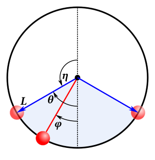
Figure 1: Simple Pendulum
Consider the simple pendulum shown in figure 1. The center-of-mass moves along a circle of radius L. The instantaneous position is given by the angle φ.
We are interested in the pendulum’s period of oscillation, denoted T. Pendulums have been used for timekeeping since Day One of modern science, and have been used to symbolize physics itself.
The period depends on the length of the pendulum (L) and on the local acceleration of gravity (g), both of which we assume are well-known and constant.1
We need to look closely at the dependence of the period on the amplitude of the oscillation, θ. On the one hand, the period is “nearly” independent of amplitude when the amplitude is small. On the other hand, a very good pendulum clock keeps time to about 0.1 ppm, so even a weak dependence is significant to horologists. Even in the introductory physics lab, it is easy to get into the regime where this dependence affects the measurements.
Here is a very useful formula for the period T. It is exact, easy to remember, and easy to use:
As derived in section 5,
| (1) |
where agM() is the arithmetic-geometric mean, as discussed in detail below. It splits the difference between the familiar arithmetic mean and geometric mean. It can be calculated very efficiently. Forsooth, it is easier to calculate agM() from scratch that it is to calculate cos() from scratch.
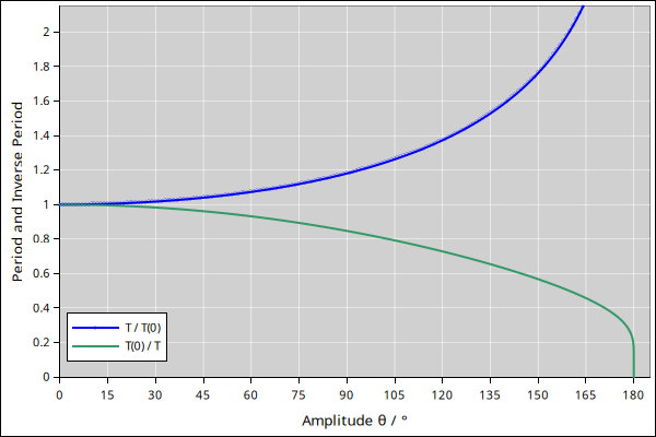
Figure 3 shows how the period depends on amplitude.
Table 1 provides similar information in tabular form, namely the depencence of period on amplitude:
| θ | T / T0 | |
| 0 | 1 | |
| 15 | 1.0043 | |
| 30 | 1.01741 | |
| 45 | 1.03997 | |
| 60 | 1.07318 | |
| 75 | 1.11896 | |
| 90 | 1.18034 | |
| 105 | 1.26221 | |
| 120 | 1.37288 | |
| 135 | 1.52795 | |
| 150 | 1.7622 | |
| 165 | 2.18544 | |
(See equation 48 for a version of equation 1 with better numerical stability in extreme cases.)
(Beware: In the literature there are dozens of formulas for approximating the period, using power series or whatever, but these are almost never useful, because the exact expression in equation 1 is simpler and better.)
Important remark: There area hundreds, maybe thousands of references that say there is no closed-form solution for the period of a pendulum, except in the small-angle approximation. They analyze small-angle case and then don’t even try to analyze larger angles. They just give up.
The point is, I consider equation 1 to be a perfectly respectable closed-form solution. The agM is perfectly well defined and easy to evaluate. Forsooth, it is easier to evaluate the agM from scratch than evaluate the cosine from scratch.
The equation of motion leads to a complete elliptic integral of the first kind. Such things crop up fairly often in math and physics. They have an undeserved reputation for being hard to deal with. If you encounter one, don’t give up. Evaluate it in terms of the agM.
There’s nothing particularly new about this. Gauss figured out how to evaluate elliptic integrals via the agM about 200 years ago. The work wasn’t published until some decades later, but still, there’s been plenty of time for the idea to spread. It’s mentioned in Abramowitz and Stegun (1964), including in the table of contents.2 Back before everything was available online, generations of physicists relied on that book. Also, the Wikipedia page for “elliptic integral” has mentioned the agM since the second edit, more than 20 years ago (March, 2002).3 There’s also a nice AJP article from 2008, discussing the agM and its application to pendulums.4 So it’s not a big secret.
Suppose we are given two numbers, a0 and b0, and we wish to find their arithmetic-geometric mean, denoted agM(a0, b0). Then we define a sequence of values, for all i≥0:
| (2) |
This is interesting because the sequence converges very quickly. After a few interations, ai is equal to bi for all practical purposes, and their shared value defines the agM.
Equivalently, we can define the agM recursively:
| (3) |
We remark that the agM has the following properties, which you would expect any sort of average to have:
| (4) |
Furthermore, the agM sequence has the wonderful property that for all i (except maybe i=0),5 ai is an upper bound on the final answer, and bi is a lower bound.
| (5) |
This means you always know how well converged the sequence is. This is unlike most sequences and series, where you have to do extra work to figure out how well converged things are.
Some c++ code to evaluate the agM can be found in section 9.
So far we have merely asserted equation 1. Let’s see if we can derive it.
Starting from the basic equations of motion, we can derive a formula that expresses the period of oscillation (T) in terms of a complete elliptic integral of the first kind. The derivation is spelled out in section 5.
| (6) |
where for a pendulum a0=1 and b0=cos(θ/2). By symmetry, we can also write this as:
| (7) |
which doesn’t tell us much we didn’t already know, but makes the geometric interpretation more clear. The RHS is the average of 1/r, averaged over all angles, where r is the radius of an ellipse centered at the origin with semi-major axis a0 and semi-minor axis is b0.
To make progress, we need a way of evaluating the integral. You could do it numerically (using Runge-Kutta or whatever), but there is a cleverer way.
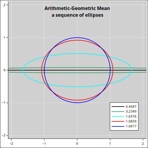
Key idea: Suppose we have a sequence of ellipses, all with the same average 1/r, and suppose the sequence rapidly converges to an ellipse that is circular. Such a sequence is shown in figure 4.
The average 1/r for a circle is obvious. Game over, you win.
The only remaining task is to find a suitable sequence of ellipses. It turns out that the ai and bi defined by equation 2 do the job very nicely.
Specifically: In equation 7, we make the following substitution:6,7
| (8) |
when we turn the crank,7,8 we find that
| (9) |
where the ai and bi have the same meaning as in equation 2. By iterating this process, we find that T/T0 converges to 1/agM(a, b), as advertised (i.e. equation 1).
In figure 4 the red ellipse is of particular relevance. It represents agM(1, √½), which is the starting point for evaluating T/T0 when the amplitude is θ=90∘. The dashed blue circle is an accurate representation of the final answer, T0/T=0.8472, obtained by two iterations of the agM algorithm.
The literature is overflowing with complicated approximations to the elliptic integral. Most of these are worthless, because the exact expression equation 1 is easier to understand, and easier to use.
However, sometimes you can improve your intuition by looking at a low-order expansion in the neighborhood of the limiting cases: small amplitude (θ near zero) and large amplitudes (η near zero).
Here’s a quick-and-dirty approximation, valid when θ is small:
| (10) |
Here’s a much more accurate approximation, sometimes useful if you’re using a spreadsheet that can do trig functions and square roots, but can’t execute imperative iterative code (as in section 9). It is equivalent to doing one 1.5 iterations by hand, algebraically (as in equation 14):
| (11) |
This is of limited utility, because even with a spreadsheet, even if you can’t do arbitrarily many iterations, you can still do enough interations to obtain very high accuracy, by directly applying the definition of agM. If necessary, add a couple of columns to the spreadsheet, to hold the intermediate ai and bi.
Let’s compare these two approximations to the exact value when θ is 45∘:
| (12) |
So even the quick-and-dirty approximation (equation 10) is in the right ballpark. For smaller amplitudes, its accuracy is better.
For larger amplitudes, or if you need more accuracy, don’t bother using a power series with more terms. Instead, use more iterations of the agM algorithm. Equation 11 is accurate within 20 ppm all the way out to θ=90∘.
Details: To derive equation 10, start with equation 1 and expand everything to lowest order:
| (13) |
To derive equation 11, the key idea is this: Directly using the definition of agM, peform the iterations using algebraic variables (rather than numbers). That gives us:
| (14) |
It’s rarely necessary to continue the process beyond this point, but you can if you want. Explicit expressions are given in reference 4.
We now consider the case of large amplitudes, where θ is large and the supplementary angle η approaches zero.
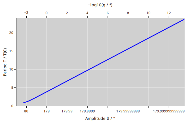
In this case, the period approaches infinity. However, the approach is remarkably slow, as shown in figure 5. In fact, for η near zero, the period is proportional to the logarithm of η.
In the figure, note that each tick mark in the horizontal direction represents two orders of magnitude of change in η. Here’s a supplement to table 1, quantifying the large-angle behavior.
| θ / ∘ | T / T0 | η / ∘ | ||
| 80 | 1.13749 | 102 | ||
| 170 | 2.43936 | 101 | ||
| 179 | 3.90107 | 100 | ||
| 179.9 | 5.36687 | 10−1 | ||
| 179.99 | 6.83274 | 10−2 | ||
| 179.999 | 8.29861 | 10−3 | ||
| 179.9999 | 9.76448 | 10−4 | ||
| 179.99999 | 11.2304 | 10−5 | ||
| 179.999999 | 12.6962 | 10−6 | ||
| 179.9999999 | 14.1621 | 10−7 | ||
| 179.99999999 | 15.628 | 10−8 | ||
| 179.999999999 | 17.0938 | 10−9 | ||
| 179.9999999999 | 18.5597 | 10−10 | ||
| 179.99999999999 | 20.0256 | 10−11 | ||
| 179.999999999999 | 21.4914 | 10−12 | ||
| 22.9573 | 10−13 | |||
| 24.4232 | 10−14 | |||
| 25.8891 | 10−15 | |||
| 27.3549 | 10−16 | |||
| 28.8208 | 10−17 | |||
| 30.2867 | 10−18 | |||
| 31.7525 | 10−19 | |||
| 33.2184 | 10−20 | |||
| 34.6843 | 10−21 | |||
| 36.1502 | 10−22 | |||
| 37.616 | 10−23 | |||
| 39.0819 | 10−24 | |||
| 40.5478 | 10−25 | |||
| 42.0136 | 10−26 | |||
| 43.4795 | 10−27 | |||
| 44.9454 | 10−28 | |||
| 46.4113 | 10−29 | |||
| 47.8771 | 10−30 | |||
| 49.343 | 10−31 | |||
| 50.8089 | 10−32 | |||
| 52.2747 | 10−33 | |||
| 53.7406 | 10−34 | |||
| 55.2065 | 10−35 | |||
| 56.6724 | 10−36 | |||
| 58.1382 | 10−37 | |||
| 59.6041 | 10−38 | |||
| 61.07 | 10−39 | |||
| 62.5358 | 10−40 | |||
Here is an interesting expression for agM(1,b), valid when b is small:9
| (15) |
This is useful because it illuminates the theory. It shows that the logarithmic divergence in figure 5 is not a fluke. In exceedingly rare cases it is useful in numerical calculations, where b is so small that it cannot accurately be represented by a floating-point number.
In particular, here’s an amusing exercise that requires more theorizing than computing: Ideally, if you balance a pencil so that it is vertical, it should stay there for a very long time before falling over. Using equation 15 (or otherwise), estimate how hard it would be to balance a pencil so precisely that it takes at least 20 seconds to fall over. (Assume the tip is sharpened so that its radius of curvature is negligible.)
Let’s derive equation 1.
We start by considering the total energy, which we take to be a constant,1 denoted E.
The kinetic part of the energy is:
| (16) |
At this point we invoke the oscillator assumption.1 That is, we assume that it’s an oscillator, not a rotor. In other words, it doesn’t have enough energy to flip over the top and keep going in the same direction. The turnaround occurs at an angle θ, as shown in the diagram, at which point the kinetic energy is zero. At other points in the swing, the potential energy differs in proportion to the difference in height, so the kinetic energy must do the same.
| (17) |
Note that we did not directly use Newton’s laws of motion. The force law would have given us an equation involving the second derivative. Here we used energy concepts (not known in Newton’s day) to obtain an equation involving the square of the first derivative, which saves us a couple of steps and makes the physical significance of equation 17 more clear.
Let’s integrate both sides of equation 17. Integrating from bottom dead center to the turning point gives us a time equal to one quarter of the oscillation period (T):
| (18) |
We are about to show that equation 18 can be written as:
| (19) |
where
| (20) |
which is the textbook standard form of the complete elliptic integral of the first kind with modulus k, denoted K(k). For our pendulum, the modulus is:
| (21) |
We can also rewrite the period as:
| (22) |
or equivalently
| (23) |
where the integral in equation 22 (not including the 2/π out front) is the standard two-argument Cayley form of the complete elliptic integral of the first kind. For the pendulum we have:
| (24) |
Equation 23 has a nifty geometric interpretation: The RHS is just the average of 1/r, averaged over all angles, as we go around an ellipse with semi-major axis a and semi-minor axis b. We have already used this idea in section 3.
This subsection is mostly routine algebra (although there is some trickery in equation 27). Feel free to skim, or skip ahead to section 6.
We can rewrite the trig functions in terms of the squares of of trig functions, using the double-angle identities, which are valid for any angle α:
| (25) |
This makes the integral look a little more “elliptical”:
| (26) |
It is slightly annoying to have θ appear both in the integrand and in the limit of integration. We can fix that, and bring the integral into a more conventional form, using the following substitution:
| (27) |
The idea is that at the turning point, where φ=θ, we have sin(u)=1 and u=π/2, which is a constant, independent of θ. The substitution is also motivated by the appearance of the square of sin(u) inside the square root. Most importantly, the substitution is motivated by 20/20 hindsight. Clever people have been down this road before, so we know where it leads. To make use of the substitution, we need its derivative:
| (28) |
So the whole integral becomes:
| (29) |
where we recognize the integral as a complete elliptic integral of the first kind.10,8 In our case the modulus is k=sin(θ/2) or equivalently the parmeter is m=k2=sin2(θ/2).
When the amplitude goes to zero, the integral is trivial to evaluate. This gives us:
| (30) |
which allows us to write an important result. The RHS of equation 31 is the standard form of the complete elliptic integral of the first kind.
| (31) |
To obtain the two-argument Cayley form, we replace the 1 in equation 31 with sin2 + cos2.
| (32) |
where for the pendulum we have a=1 and b=cos(θ/2). These results are discussed and applied back in section 5.2
We wish to prove equation 9, which we restate here:11
| (33) |
using the notation for ai and bi as defined in equation 2.
It’s not obvious how to proceed, so we rely on Gauss to help us get started. We make the following substitution:
| (34) |
In some sense, that’s all you need to know. The rest is just algebra. Pages and pages of algebra.
Remark: When u is zero, u′ is also zero. Also, when u is π/2, u′ is also π/2. It pretty much has to be this way, on account of the symmetry of the ellipses in figure 4.
We restate equation 32 with a trivial modification, and then organize the rest of the work in three stages.
| (35) |
Stage 1: In section 6.2, we will show that the cosine factor is:
| (36) |
where D is the denominator of equation 34, namely:
| (37) |
In equation 36 we are happy to see a1 and b1. The square root can be visualized as the radius of an ellipse with semi-major axis a1 and semi-minor axis b1, which is concept we have seen a couple of times already.
Stage 2: In section 6.3, we will show that the radius factor is:
| (38) |
Stage 3: In section 6.4, we will show the numerator of equation 35 is:
| (39) |
We plug these subsidiary results into equation 35, and almost everything cancels out:
| (40) |
just as advertised.
The following three subsections are just algebra. They’re not very interesting. They are included mainly to reassure you that you could do the calculations if you wanted. No wizardly required. The only serious wizardry was back in equation 34, along with the underlying idea of a sequence of integrals.
Feel free to skip ahead to section 7
To obtain a formula for cos(u), we start with equation 34, then multiply both sides by D and turn the crank:
| (41) |
We would like to pull out a factor of cos2(u′) on the right, to go with the cos2(u) on the left. And once again we are motivated by 20/20 hindsight. The calculation continues:
| (42) |
| (43) |
Next, let’s work out the other factor in the denominator of equation 35, namely the square root, i.e. the “old” radius. In that factor, we use equation 34 to plug in for for sin(u), and use equation 43 to plug in for cos(u). Then turn the crank:
| (44) |
The RHS is a perfect square, so we are left with an expression that is a lot simpler than the steps that led to it:
| (45) |
Last but not least, we need to deal with the numerator in equation 35. In particular, we need to express it in terms of u′. We do that by restating equation 34 and differentiating both sides:
| (46) |
So:
| (47) |
Here’s some stuff that non-experts don’t need to know, but may find amusing.
Equation 1 is mathematically correct and is directly usable in all but the most extreme situations. However, when doing floating-point calculations, roundoff becomes a problem when the amplitude θ is very large, specifically when the supplementary angle η is very small compared to 1. In such situations you should use the last line of equation 48, which is mathematically equivalent but numerically more robust. It remains usable down to η=10−100 and beyond.
| (48) |
This was useful for preparing figure 5 and table 2.
In the sequence that defines the agM, you can move backwards using the expressions:12
| (49) |
Note: In such a series, ai ≥ bi for all i (except possibly i=0),5 as a direct consequence of the definition.
Gauss’s Constant: The reciprocal of agM(1,√2) is known as Gauss’s constant, G≈0.834627. It shows up in various contexts in analysis.13 The period for a pendulum when the amplitude is 90∘ is T/T0=√2 G.
Galileo’s Constant: The quarter-period is the time it takes a pendulum to fall to the middle, starting from rest at some angle θ. This is proportional to the time it takes for an object to fall a distance L, starting from rest, where L is the length of the pendulum. For small amplitudes, this is a universal constant, namely π / √8. Stillman Drake calls this Galileo’s constant,14 although I’m not sure anybody else does. Galileo had to determine this quantity experimentally, since the necessary theory (Newtonian mechanics) hadn’t been invented yet.
Our calculations are based on the following assumptions.
| Oscillator: We assume that the pendulum is actually pendulous, i.e. it hangs down. | In other words, we assume it is an oscillator, not a rotor. It doesn’t have enough energy to flip over the top and keep going in the same direction. |
| Stable conditions: We assume the pivot is well supported and not wobbling. We assume the length L is well-known and not changing. Similarly we assume the local acceleration of gravity g is well-known and not changing. | Beware that g varies from one geographic location to another, by an amount that is easily measurable with a good pendulum clock. |
| Moving in a single vertical plane. | It is certainly possible to have a spherical pendulum. When the amplitude is small, this is not too bad. In the special case of a conical pendulum, where the bob moves in a horizonal circle, this is not to bad. However, the general case is very complicated. |
| Lossless: We neglect friction of all kinds. In other words, the system energy E is constant. |
| Airless: We neglect buoyancy, breezes, and all other static and dynamic contributions from the air. |
| Simple pendulum. | That is, not a compound pendulum, i.e. not a pendulum attached to another pendulum. |
| Rigid: In cases where the amplitude θ is larger than 90∘, we assume the bob is connected to the pivot by a rigid rod. | You can use a string for small angles, but not large angles, because it would go slack. |
| Bob Only: We assume the pendulum has the conventional design, so that the mass of the connecting rod is negligible compared to the mass of the bob. | For an arbitrary distribution of mass, deriving the equation of motion would be slightly more complicated. The potential energy would still be proportional to −cos(φ), and kinetic energy would still be proportional to (dφ/dt)2, so the calculation runs parallel the one in section 5; you just have to figure out the proportionality factors. |
| Non-Thermal: We ignore thermal fluctuations. | In the classical approximation, if the mass is large enough, the friction is small enough, and the temperature is low enough, the thermal fluctuations are negligible. |
| Classical: In rough terms, we assume the system is “classical” in the sense that we don’t need to worry about relativistic effects. | In more precise terms, everything is subject to the laws of relativity. Momentum is first order in v/c, and kinetic energy is second order in v/c, so what we are really saying is the third-order (and higher) terms are neglgible. To put it another way, phenomena that were well known prior to 1887, prior to Michelson-Morley, are considered classical. |
| Similarly, classical means we neglect general relativity. This is an excellent approximation. | Again, everything is subject to the laws of general relativity. In practice, we don’t need to worry about it when the distances are not enormously large, and the gravitational fields are not enormously strong. |
| Classical also means we neglect quantum effects. This is not an entirely trivial assumption. QM places some rather strict bounds on how long you can make a pencil balance on end. | Again, everything is subject to the laws of QM. Quantum mechanics contains, predicts, and explains classical mechanics — but not vice versa. In practice, if the bob is massive enough and you don’t look too closely, the equations of classical physics are good enough. |
| In the definition of agM(a, b) we assume that a and b are positive real numbers. For the pendulum we are considering, this is automatically true, as a consequence of the other assumptions. | The agM function can by analytically continued to arbitrary complex numbers. This has some interesting properties, but is of no help in analyzing the pendulum. |
// <*><*><*><*>  arithmetic-geometric-mean.c  <*><*><*><*>
#include <cmath>
#include <stdexcept>
#include "arithmetic-geometric-mean.h"
using namespace std;
static double const qnan = numeric_limits<double>::quiet_NaN();

// Simple version of the arithmetic-geometric mean.
// A first step, for edification.
// Not industrial strength.
double agM_simple(double ai, double bi) {
  int maxit(20);
  for (int iter=0;;) {
    if (ai == bi) break;
    if (iter >= maxit) throw runtime_error("agM didn't converge");
    double anew = (ai+bi)/2.;
    double bnew = sqrt(ai*bi);
    ++iter;               // count # of iterations needed
    if (fabs(anew-bnew) >= fabs(ai-bi)) {
// previous values (ai,bi) were just as good, maybe better
      break;
    }
    ai = anew;
    bi = bnew;
  }
  return ai;
}

// Fancy version.
// More defensive about extreme cases and out-of-bounds cases.
//
// Some typical usages, among others:
// Simplest case:
//   mean = agM(a,b);
//   mean = agM(a);     // same as agM(a,1.)
// More information is available from the structured object:
//   AGM foo(a,b); mean = foo.ai;  iter = foo.iter;
//   AGM foo; mean = foo.agM(a,b); iter = foo.iter;

double AGM::agM(double const a0, double const b0) {
  ai = a0;
  bi = b0;
  iter = 0;
  if (bi == 0) return (ai=bi);
  if (ai == 0) return (bi=ai);
  if (ai-ai != 0) return (bi=ai);      // defend against nan and inf
  if (bi-bi != 0) return (ai=bi);
  if (bi < 0) return ai=bi=qnan;
  if (ai < 0) return ai=bi=qnan;
  for (;;) {
    if (ai == bi) break;
// check for badness /after/ checking for goodness:
    if (iter >= maxit) throw runtime_error("agM didn't converge");
// Two separate square roots, to defend against the possibility
// that the product of ai*bi would cause overflow or underflow.
// Separation slows down the typical (non-nasty) case, and I do
// know how to optimize it, but overall the routine is so efficient
// that optimizing it would be silly.
// FWIW: In non-nasty cases the root of the product may differ from
// the product of the roots by 1 ULP (unit in the last place).
    bnew = sqrt(ai) * sqrt(bi);
    anew = (ai+bi)/2.;
    ++iter;               // count # of iterations needed
    if (fabs(anew-bnew) >= fabs(ai-bi)) {
// previous values (ai,bi) were just as good, maybe better
      break;
    }
    ai = anew;
    bi = bnew;
  }
  return ai;
}

// maxit is 20 because 15 iterations are needed
// when a=1e300 and b=1e-300
//
// except for maxit, these are all out-of-bounds values,
// to make sure that anybody who uses them initializes them.
AGM::AGM()
 : maxit(20), iter(10*maxit), ai(-1.), bi(-1), anew(-1.), bnew(-1.) {}

AGM::AGM(double const _a, double const _b) : AGM() {
  agM(_a, _b);
}

// not a class member:
double agM(double const a0, double const b0) {
  return AGM(a0, b0).ai;
}

// <*><*><*><*>  arithmetic-geometric-mean.h  <*><*><*><*>
#pragma once
double agM_simple(double a0, double b0);
struct AGM {
  int maxit;
  int iter;
  double ai, bi, anew, bnew;
  double agM(double const _a, double const _b=1);
// constructors:
  AGM();        // doesn't do any work
  AGM(double const _a, double const _b=1);
};

// not a class member:
double agM(double const a0, double const b0=1);