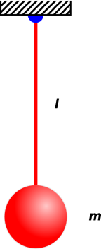
Figure 1: Simple Pendulum
Dimensional analysis is a widely known, highly useful technique. Dimensional analysis can be considered a simplified type of scaling argument, as discussed in reference 1.
By way of background, note that dimensions are not the same as units. This becomes particularly clear when you consider dimensionless units, as discussed in reference 2. In this document, we are talking about dimensions, not units.
Let’s start with the following simple scenario: Simplicio places a one-foot-long ruler into a one-gallon jug and observes that it just fits. He concludes:
| (1) |
You can instantly detect that equation 1 is dimensionally unsound. A gallon is a measure of volume, so the RHS of this equation has dimensions of length cubed, where as the LHS has dimensions of plain old length.
The rule is that any valid equation must have the same dimensions on both sides. This rule is very powerful and very easy to apply. You should routinely use it to check your equations.
Some notation (involving square brackets) to help you perform such checks will be presented in section 4.
Elementary dimensional analysis is binary: It tells us, yes or no, whether a given equation is dimensionally consistent.
Scaling arguments have been an important part of modern science since Day One (reference 3 or reference 4) and have remained important ever since.
The idea of scaling (as discussed in reference 1) is intimately connected with dimensional analysis. Specifically, we can quantify the problem by checking the scaling. In this case, try multiplying both sides of equation 1 by a factor of 2. That gives:
| (2) |
The new equation says Simplicio should be able to just fit two-foot ruler into a two-gallon jug. However, if you try it, you will find that it doesn’t work. For a linear scale factor of K, length (feet) scales like K while volume (gallons) scales like K3.
In contrast, whenever you have a dimensionally-sound equation, you will find that you can multiply both sides by some factor and get a new dimensionally-sound equation. For example, if we had gallons on one side and cubic feet on the other, it would scale correctly.
Tangential remark: The reasoning here depends on on the dimensions, not the units. Equation 1 would be dimensionally unsound even if you re-expressed it in other units.
Dimensional analysis is a subset of scaling. Sometimes you can make a scaling argument that goes significantly beyond anything you could do with dimensional analysis, e.g. the “mean free path” scaling law as discussed in reference 1.
We now turn to something more sophisticated. It should be called dimensional synthesis rather than dimensional analysis, because it is used to conjure up new equations from scratch.
As before, the key idea is that we want an equation where both sides have consistent dimensions. The new trick is that we throw in some adjustable parameters, and adjust things until we achieve consistent dimensions.
Here’s a seemingly similar question that leads to a slightly different answer. Consider a simple pendulum of length l and mass m as shown in figure 1. It is subject to a gravitational field of magnitude g.
We want to know τ, the period of oscillation. We won’t be able to find the period exactly, but we can find a scaling law, as follows:
| τ ∝ ma lb gc (3) |
The dimensions in this equation are:
| [t] = [m]a [l]b [l]c [t]−2c (4) |
where a, b, and c are (for the moment) unknowns, to be determined by dimensional analysis. We have used the fact that g has dimensions of acceleration, i.e. dimensions of length per time squared.
The square brackets in such equations are important. Symbols of the form [⋯] should be read as “dimensions of ⋯”. In this case, [t] denotes dimensions of time, [m] denotes dimensions of mass, and [l] denotes dimensions of length. In particular, [m] means m as in mass; it does not mean m as in meters of length.
Comparing dimensions on the two sides of equation 4, we get a system of three linear equations in three unknowns, namely
| (5) |
In general, you can solve such systems using Gaussian elimination, as discussed in reference 5 … In simple cases like this, you can solve this system in your head. We find that a=0, b=1/2, and c=−1/2. Plugging in, that tells us that
| (6) |
We see that the period scales like the square root of the length. This is a famous result, dating back to 1638 (reference 3).
Section 4.1 makes it seem like you can solve physics problems without knowing any physics, just using dimensional analysis, following a mechanical procedure. Alas, this is too good to be true. In fact you need to know quite a lot of physics before you can write down equation 3.
For starters, the length of the pendulum (l) is not the only relevant quantity with dimensions of length; there is also the amplitude of the oscillation.
It turns out that we can get away with omitting the amplitude from equation 3 if the amplitude is small, because the period of oscillation is independent of the oscillation. It only works for smallish oscillations, so equation 3 must be considered an approximation.
As soon as we consider the higher-order terms, the period is no longer independent of amplitude. This dependence is not well described in terms of power-law scaling.
There are other quantities that one might need to take into account. What about friction? What about the elasticity of the rod? What about the speed of sound? What about the speed of light? What about the radius of the earth? There is no fundamental law that says these things are negligible, and indeed one can find situations where they are not negligible. So in some sense it comes down to a question of engineering: It is possible to construct a pendulum where the various correction terms don’t matter, especially if you don’t look too closely. (On the other hand, if you want to build a high-precision pendulum clock, you need consider a great many nonidealities, accounting for them in great detail.)
One of the variables we thought was possibly relevant in equation 3 turned out to be not relevant. Equation 6 tells us that the period scales like mass to the zeroth power. We need to check that this makes sense, physically. Indeed it does make sense, as a consequence of the equivalence principle: if we increase the mass, the gravitational force increases, but the inertia also increases, so the acceleration stays the same. The equation of motion can be written in such a way that it depends on acceleration directly (not on mass or force separately).
This is significant, because as a general rule, if there are too many variables in an equation like equation 3, there will not be a unique solution. Therefore irrelevant variables should be omitted from the dimensional-synthesis equation.
Let’s consider the following scenario: We have a wave traveling across a large body of water such as the ocean. The wave has a well-defined wavelength, i.e. the wave is monochromatic. The wavelength is reasonably long (20 cm or more), but the wavelength is short compared to the depth of the water. We want to know the speed of propagation of the wave.
Intuition says that the only relevant physical parameters are the wavelength λ, the speed vg, the density ρ, and the gravitational field strength g.
The analysis proceeds pretty much in parallel to the analysis in section 4.1 and section 4.2. We start with the Ansatz
| vg ∝ ρa λb gc (7) |
| [l] [t]−1 = [m]a [l]−3a [l]b [l]c [t]−2c (8) |
where a, b, and c are (for the moment) unknowns, to be determined by dimensional analysis.
From this we obtain a system of three linear equations in three unknowns:
| (9) |
This is easy to solve. We obtain a=0 and b=c=1/2. Plugging in, we find the answer is:
| vg ∝ | √ |
| (10) |
Remark: Really long waves are impressively fast; a tsunami can go 600 to 800 km per hour.
Also note that this is quite a departure from the usual introductory discussion of light waves and sound waves, where it is assumed that the speed is independent of the wavelength. Note that a wave cannot maintain its shape if different Fourier components are traveling at different speeds, so the fundamental definition of “what is a wave” must be reconsidered.
We should check that it makes sense that the density drops out of the answer. Indeed this does make sense, for much the same reason that the mass dropped out in section 4.2. The restoring force (which speeds up the wave) is proportional to the gravitational force, which depends on ρ, while the inertia (which slows down the wave) also depends on ρ in the same way.
Let’s consider a new scenario: We have a wave with a well-defined wavelength, i.e. a monochromatic wave. The wavelength is short in absolute terms (2 mm or less), and short compared to the depth of the water. We want to know the speed of propagation of the wave.
Intuition says that the only relevant physical parameters are the wavelength λ, the speed vc, the density ρ, and the surface tension s.
The analysis proceeds pretty much in parallel to the analysis in previous sections. We start with the Ansatz
| vc ∝ ρa λb sc (11) |
| [l] [t]−1 = [m]a [l]−3a [l]b [m]c [t]−2c (12) |
where a, b, and c are (for the moment) unknowns, to be determined by dimensional analysis.
We have used the fact that the surface tension has units of force per unit length, and force has units of [m] [l] / [t]2 (as you can infer from the equation F=ma or in innumerable other ways).
From this we obtain a system of three linear equations in three unknowns:
| (13) |
This is easy to solve. We obtain c=1/2 and a=b=−1/2. Plugging in, we find the answer is:
| vc ∝ | √ |
| (14) |
You can check that the restoring force (s) makes the wave go faster, while the inertia (ρ) makes the wave go slower.
We see the speed of capillary waves scales inversely like the square root of wavelength, which is from section 4.3, where the speed of gravity waves scaled directly like the square root of wavelength.
Of course it is possible to derive an actual equation (not just a scaling relationship) for the speed of waves on water. See reference 6.
Let’s consider the following scenario: We have a wave traveling across a shallow body of water. The wave has a well-defined wavelength, i.e. the wave is monochromatic. The wavelength is long compared to the depth (d) of the water, and long enough that the surface tension contribution is negligible.
By analogy to section 4.3, you should not be surprised to hear that the speed of propagation scales like the square root of the depth. In particular,
| vs ∝ | √ |
| (15) |
We can use equation 16 as an example. It expresses the valid and important point that molar entropy can be measured either in units of bits per particle, or in units of joules per kelvin per mole.
| (16) |
Someone who looks at this equation without understanding it will get into trouble, because superficially it appears the LHS has different dimensions from the RHS. A more skillful practitioner will realize that the energy per particle will necessarily scale like the temperature. The physics guarantees it. So even though the BIPM in Paris does not define the kelvin in terms of joules per particle, the physics says the kelvin scales like joules per particle, and scaling is what matters, as discussed in reference 1.
Remember that dimensional analysis is not magic. It is not axiomatic. It is not some God-given 11th commandment. Instead, it is a logical corollary of the scaling laws. So if the units are telling you one thing and the scaling is telling you another, trust the scaling.
The starting point and ending point for any discussion of equation 16 must recognize that it is physically sound. It scales correctly. Whether or not it is dimensionally sound doesn’t matter. If you want to make it dimensionally sound, you don’t change equation 16; you change your notion of “dimensions” so that dimensions of temperature are interchangeable with dimensions of energy per particle.
From this we conclude that two dimensions might or might not be equivalent, depending on context. A given expression might or might not be dimensionally sound, depending on context.
As always, keep in mind that there is more to physics than dimensional analysis. You need to know the physics of the actual situation to know whether it is possible to mix time and distance (as in relativity) – or not possible to mix them (as at the track meet).
Not everything that is nominally dimensionless behaves as a dimensionless quantity should.
Here’s what we expect: As discussed above, if we have a quantity Y with dimensions of length cubed, and we scale up every length in the system by a factor of five, in simple cases we expect Y to scale up by a factor of five cubed. By the same token, if we have a quantity Z that is dimensionless, our first guess is that it will scale like length to the zeroth power, i.e. that it will be unchanged if we scale up the length.
As mentioned in section 5.1, dimensional analysis is usually just a stand-in for a scaling argument, and if the dimensions are telling you one thing while the scaling is telling you another, you should trust the scaling.
Here’s an example of what can go wrong: Suppose Simplicio defines a new quantity called longivity, which is calculated by dividing the length by one inch. The longivity of a violin string is about 12. Longivity is nominally dimensionless, by construction. However, it does not behave as a dimensionless quantity should. If we scale up every length by a factor of 3, we (approximately) convert the violin into a string bass. The longivity of the strings goes up by a factor of 3. In other words, longivity has nominal dimensions of length to the zeroth power, but scales like length to the first power.
I use the term illegitimate dimensions to refer to any situation where a quantity has nominal dimensions that conflict with its scaling behavior. (Most commonly, illegitimate dimensions are used to make a quantity appear dimensionless, but there are other possibilities. In theory, something that scales like volume could illegitimately be given units of length.)
Usually, when such a quantity is defined, some sort of explicit, arbitrary unit appears in the definition, such as the inch that appeared in the definition of longivity.
By way of contrast, it is legitimate to form a dimensionless quantity by dividing one physically-relevant thing by another physically relevant thing. For example, the aspect ratio of a wing is the span divided by the chord. The aspect ratio is a legitimate, relevant, and useful quantity.
An interesting example that straddles the border between illegitimate and legitimate concerns the activity and equilibrium quotient of chemical reactions, as discussed in reference 1.
The sort of advanced dimensional analysis discussed in section 4 is nowhere near being foolproof. In skilled hands, dimensional analysis is a method for finding the right answer quickly ... but in unskilled hands it can be a method for finding the wrong answer quickly, which is definitely not a good thing.
As an ultra-simple example, consider the fact that energies, Lagrangians, and torques all have the same dimensions. So, if you tried to equate a torque with a Lagrangian, the equation would be nonsense but it would pass the dimensional test. This is an example of a false positive dimensional test.
As a more realistic example, if we tried to combine section 4.3 and section 4.4, including the effects of both gravity and surface tension, we would wind up with three equations in four unknowns, and we would be stuck.
In such a situation, it is possible to get un-stuck, but doing so requires a good grasp of the physics of the situation. Often this boils down to knowing which variables are relevant. Continuing the wave example, if we include the effects of both gravity and surface tension, we would be able to construct the following dimensionless quantity:
| (17) |
Similarly, if we tried to combine section 4.3 and section 4.5, we would encounter the dimensionless quantity
| (18) |
When you have a dimensionless quantity running around, you can multiply one side of an equation (such as equation 14) by that quantity raised to any power you want, and the result will be dimensionally sound. If you blindly apply the dimensional analysis formalism to such a situation, you can get any answer you want, including innumerably many wrong answers. The solution to this problem lies outside the scope of dimensional analysis. You need more powerful tools (such as scaling laws) that allow you to bring in more of the physics, as discussed in reference 1.
The combination of section 4.3 and section 4.5 provides a nice example of the power and the limitations of dimensional analysis. It turns out that the shallow-water case can be solved exactly by elementary methods. If you do the full-blown calculation, you will find that
| vs = | √ |
| (19) |
which is an equality, in contrast to equation 15 which was merely a proportionality.
The calculation for deep-water waves is very much more complex. Instead of doing the calculation, we rely on qualitative physical arguments to tell us that equation 19 cannot remain valid in deep water. It would be very weird if the wavefunction of the wave could extend to arbitrarily great depths. There must be some sort of cutoff, some sort of limit as to how deep the influence of the wave extends. If the water is deep enough, the depth must be immaterial. The only remaining length-scale in the problem is the wavelength, so the cutoff must scale like the wavelength, and the speed must then scale according to equation 10.
Dimensional analysis, like many tools, mostly multiplies your existing skills, rather than merely adding to them. If you don’t know anything, dimensional analysis isn’t going to help you. On the other hand, the more you know, the more powerful dimensional analysis and scaling arguments become.
Note that in this context, the dimensionless groups such as appear in equation 17 and equation 18 are traditionally given names of the form π with a subscript, which is the basis for the name of the “Buckingham pi” theorem (reference 7).
Rather than talking about what dimensional analysis can’t do, it would be more constructive to talk about what scaling arguments can do. In reference 1 there are many examples of scaling laws, some of which can easily be derived using dimensional arguments, but some of which cannot (such as the distance to the apparent horizon, and the monomer/dimer equilibrium density).
Beware that sometimes a dimension is named after a unit. There are many examples, including voltage, acreage, mileage, et cetera. This is discussed in reference 8.
Back when I was a senior in college, I was taking a course in General Relativity. The second-term final exam was a one-on-one oral exam. I showed up for my appointment at 8:00AM. I had stayed up all night. (I hadn’t been studying; I had been too busy printing a million entries for the McDonald’s sweepstakes … but that’s another story.)
The dialog went something like this:
At this point the exam was over. I had gotten two out of three questions abjectly, totally, and fundamentally wrong. And it was clear that I hadn’t studied the gravitational radiation formula. But I guess Kip figured out that anybody who could construct the formula on the spot – using nothing but dimensional analysis and scaling arguments – couldn’t be all bad. He even gave me a decent grade in the course.